The hybrid dispersion test
tests/functional/dispersion/dispersion.py checks that PHARE’s hybrid model propagates
waves at the right frequency. It loads small-amplitude waves along \(\vb{B}_0\), measures
their frequency \(\omega\) and compares it to the theoretical dispersion relation, for
16 wavenumbers spanning two decades, on two branches, for particle interpolation orders
1, 2 and 3.
checks |
\(\omega(k)\) of the whistler (R) and Alfvén/ion-cyclotron (L) branches, \(0.06 \leq k d_i \leq 4\) |
runs |
2 resolutions \(\times\) 3 interpolation orders = 6 one-dimensional runs |
cost |
about 80 s in total (Release build, one core) |
pass if |
every \(\omega\) is within 1% of the expected value, and no wave is lost |
ctest |
|
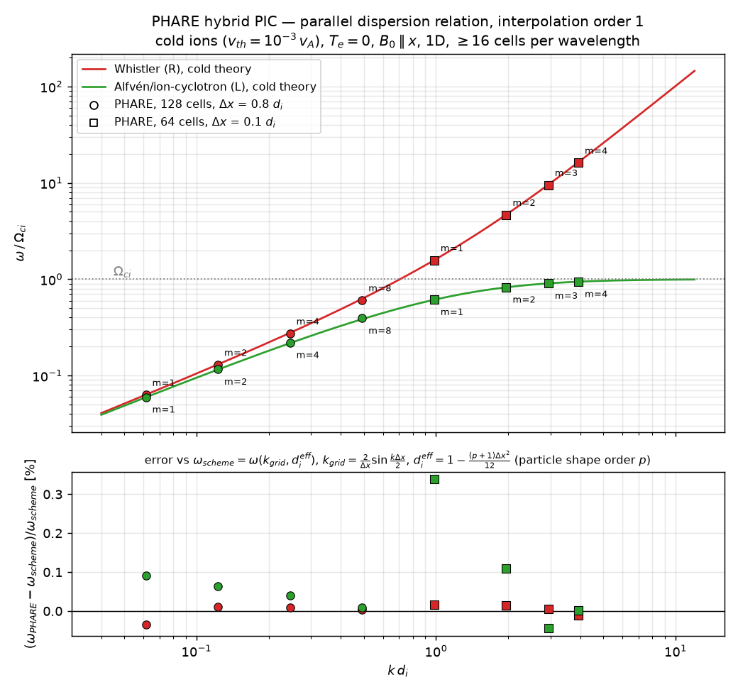
Measured frequencies (markers) against the cold-plasma theory (lines). Circles come from the coarse run (\(\Delta x = 0.8\,d_i\)), squares from the fine one (\(\Delta x = 0.1\,d_i\)). Lower panel: relative error against what the scheme should give (section 3).
1. The physics
The test uses the simplest plasma with two wave branches: cold ions, cold massless electrons (\(T_e = 0\)), and a uniform field \(\vb{B}_0 = B_0\,\vu{x}\). Waves propagate along \(x\) and are transverse. Units are the ion inertial length \(d_i\), the inverse ion cyclotron frequency \(\Omega_{ci}^{-1}\) and the Alfvén speed \(v_A\).
With the complex notation \(b = B_y + i B_z\) and \(u = v_y + i v_z\) (ion bulk velocity), the ion momentum equation and Faraday’s law with the Hall electric field reduce to
The last term is the Hall term: it is what makes the hybrid model different from ideal MHD. A mode \(b \propto e^{i(qx - \omega t)}\) obeys
\(\omega_+\) is the whistler (right-hand, R) branch: \(\omega \to k^2 d_i\) at large \(k\).
\(\omega_-\) is the Alfvén/ion-cyclotron (AIC, left-hand, L) branch: \(\omega \to \Omega_{ci}\) at large \(k\).
At small \(k\) both reduce to the Alfvén wave \(\omega = k v_A\); their gap, the Hall splitting \(\omega_+ - \omega_- = k^2 d_i\), is a direct measure of the Hall term.
Each root comes with the eigenvector \(u = -(q/\omega)\, b\): to load a pure wave of one branch, the ion velocity must be set accordingly.
2. How the test measures \(\omega\)
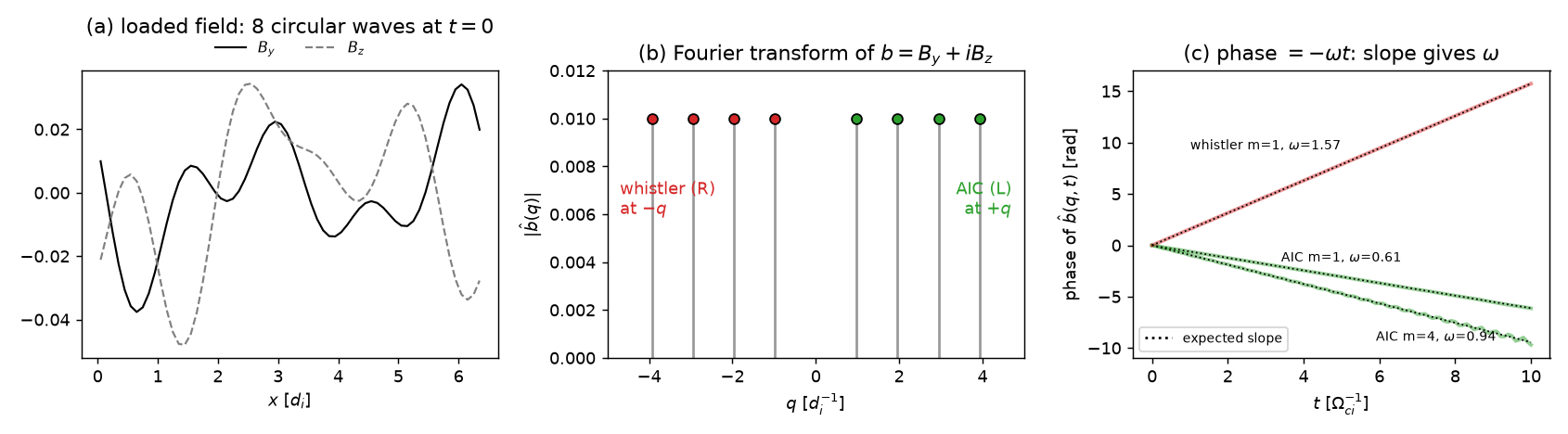
(a) The loaded \(B_y\), \(B_z\): a sum of 8 circularly polarized waves. (b) Their Fourier transform: AIC waves sit at \(+q\), whistlers at \(-q\), so each Fourier bin holds one wave. (c) The phase of each bin decreases linearly in time; the slope is \(-\omega\).
Load pure eigenmodes. For \(m = 1, 2, 4, 8\) (coarse run) or \(m = 1, 2, 3, 4\) (fine run), with \(k_0 = 2\pi/L\):
an AIC wave at \(q = +m k_0\) and a whistler at \(q = -m k_0\);
\(b = 10^{-2}\, e^{i(qx + \varphi)}\) with a fixed random phase \(\varphi\), and \(u = -(q/\omega)\, b\), so that each wave is a single eigenmode.
Run and write \(B\) every 10 steps.
Project \(b(x, t)\) on each loaded wavenumber: \(\hat b(q, t) = \frac{1}{N}\sum_j b(x_j, t)\, e^{-i q x_j}\).
Fit a straight line to the unwrapped phase of \(\hat b(q, t)\): the slope is \(-\omega\). This works with a few periods, far fewer than a time Fourier transform would need, which keeps the runs short.
Two runs cover the \(k\) range: \(L = 102.4\,d_i\) with 128 cells for \(0.06 \leq k d_i \leq 0.5\) (Alfvén regime, where the Hall splitting is small, 100 particles per cell), and \(L = 6.4\,d_i\) with 64 cells for \(1 \leq k d_i \leq 4\) (ion scales, where the branches separate, 400 particles per cell). Every wave is resolved by 16 cells or more.
Settings that matter:
hyper-resistivity is 0: its default, \(10^{-4}\), damps short waves at a rate \(\sim 10^{-4} k^4\);
ions are cold, \(v_{th} = 10^{-3}\,v_A\), so that the AIC waves stay far from the ion-cyclotron resonance;
the amplitude \(\delta B/B_0 = 10^{-2}\) must stay small: at \(3\times10^{-2}\) the AIC frequencies shift by about +3% (a nonlinear effect, growing as \(\delta B^2\)) and the AIC waves near \(\Omega_{ci}\) break up;
particle noise is therefore reduced with particles: near \(\Omega_{ci}\), with 100 particles per cell, noise is as large as the wave itself.
3. What the scheme should give
Even a perfect implementation does not reproduce (2) exactly: two discretization effects shift \(\omega\) in a known way, and the test compares against \(\omega\) corrected for both.
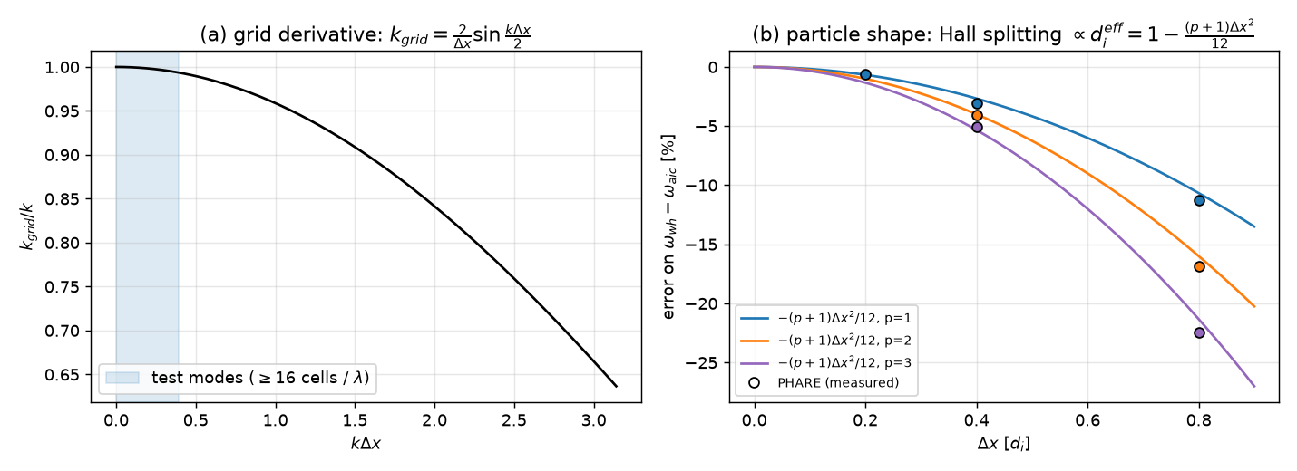
(a) Grid derivative. On the staggered (Yee) grid a derivative is a centered difference, which acts on \(e^{ikx}\) as \(i k_{grid}\) instead of \(i k\):
The whistler, \(\omega \approx k^2 d_i\), feels it twice. At 8 cells per wavelength (\(k\Delta x = 0.79\)) this alone shifts the whistler by \(-5\%\); at 16 cells by \(-1.2\%\).
(b) Particle shape. Particles deposit their moments and receive fields through a B-spline shape of order \(p\), whose spread (variance) is \((p+1)\Delta x^2/12\): an order-\(p\) B-spline is \(p+1\) top-hats of width \(\Delta x\) convolved together, each top-hat has variance \(\Delta x^2/12\), and variances add (order 1, the linear “hat”, gives \(\Delta x^2/6\)). The measured effect is that the Hall term is weakened as if
At \(\Delta x = 0.8\,d_i\) and \(p = 1\) this makes the Hall splitting 11% too small; at \(p = 3\), 21%. The effect scales as \(\Delta x^2\) (measured at \(\Delta x\) = 0.2, 0.4, 0.8) and as \(p + 1\) (measured for \(p\) = 1, 2, 3: errors in the ratio 1 : 1.49 : 2.0, against 2 : 3 : 4 = 1 : 1.5 : 2 predicted), and does not depend on the time step. Formula (4) is empirical: it fits all measurements, but has not been derived.
Note
This is a property of PHARE runs, not only of this test: at \(\Delta x \gtrsim 0.5\,d_i\) the Hall physics is weakened by ten percent or more, and more so at higher interpolation order.
The expected frequency is therefore
and with it, all 48 points (16 modes \(\times\) 3 orders) agree to better than 0.4%.
4. Pass/fail criteria and calibration
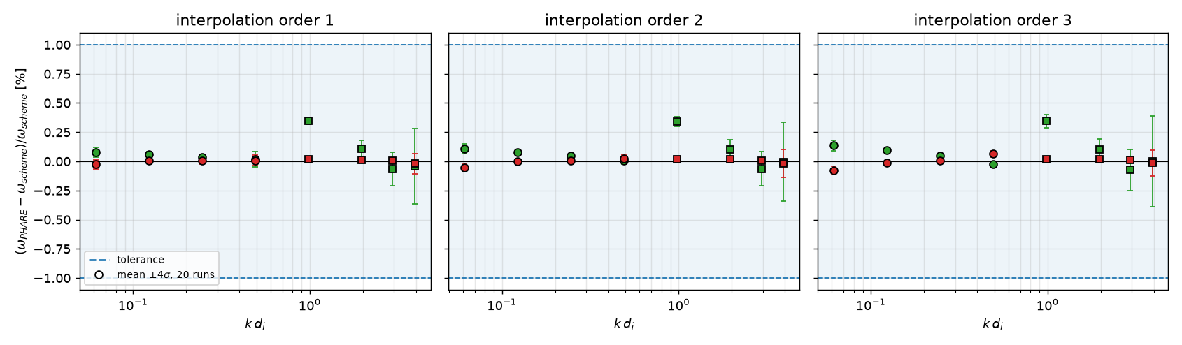
Error against \(\omega_{scheme}\) for every point, mean \(\pm 4\sigma\) over 20 independent runs (different particle draws). Dashed: the 1% tolerance.
The test fails if, for any mode:
\(|\omega_{PHARE} - \omega_{scheme}| / \omega_{scheme} > 1\%\), or
the mode’s amplitude at the end is outside \([0.3, 3]\) times its initial value (the wave was damped away or swamped by noise).
The spread comes from particle noise and is largest for the ion-scale AIC waves near \(\Omega_{ci}\). Final amplitudes stayed between 0.50 and 1.60 times their initial value. One small bias is not explained yet: the ion-scale AIC wave at \(k d_i \approx 1\) is +0.35% off in every run and at every order. Over 20 runs, the largest \(|\text{bias}| + 4\sigma\) is 0.40%, which leaves a margin of a factor 2.5 below the tolerance.
5. Running it and reading a failure
cd build && ctest -R py3_test-dispersion -V        # the three orders, in parallel with -j
# or directly, from a scratch directory
PYTHONPATH=<build>:<repo>/pyphare python3 <repo>/tests/functional/dispersion/dispersion.py [1|2|3] [low_k|high_k]
Without arguments it runs every order and both runs. It prints one table per
interpolation order and writes dispersion_o{1,2,3}.png.
what fails |
likely cause |
|---|---|
whistlers at large \(k\) |
Hall term, Ohm’s law, Faraday, or the time step |
AIC at large \(k\) |
ion pusher (gyration), moment deposit |
both branches at small \(k\) |
Alfvén speed: field or density normalization, current |
the gap between branches only |
Hall term, or the particle shape (interpolation, deposit) |
one interpolation order only |
that order’s shape functions |
amplitude out of range |
wave damped (resistivity, hyper-resistivity) or noise too large |